Studies are everywhere
I tend to read through meta-analyses to get the jist of an area of interest. For example, I might want to know, without trawling through hundreds of studies, how effective a specific type of psychotherapy is for a particular psychiatric condition. Meta-analyses are great for providing a summary of this information. I then figured, well, how can we do these analyses in R and conduct a meta-analysis and render a fancy looking forest plot.
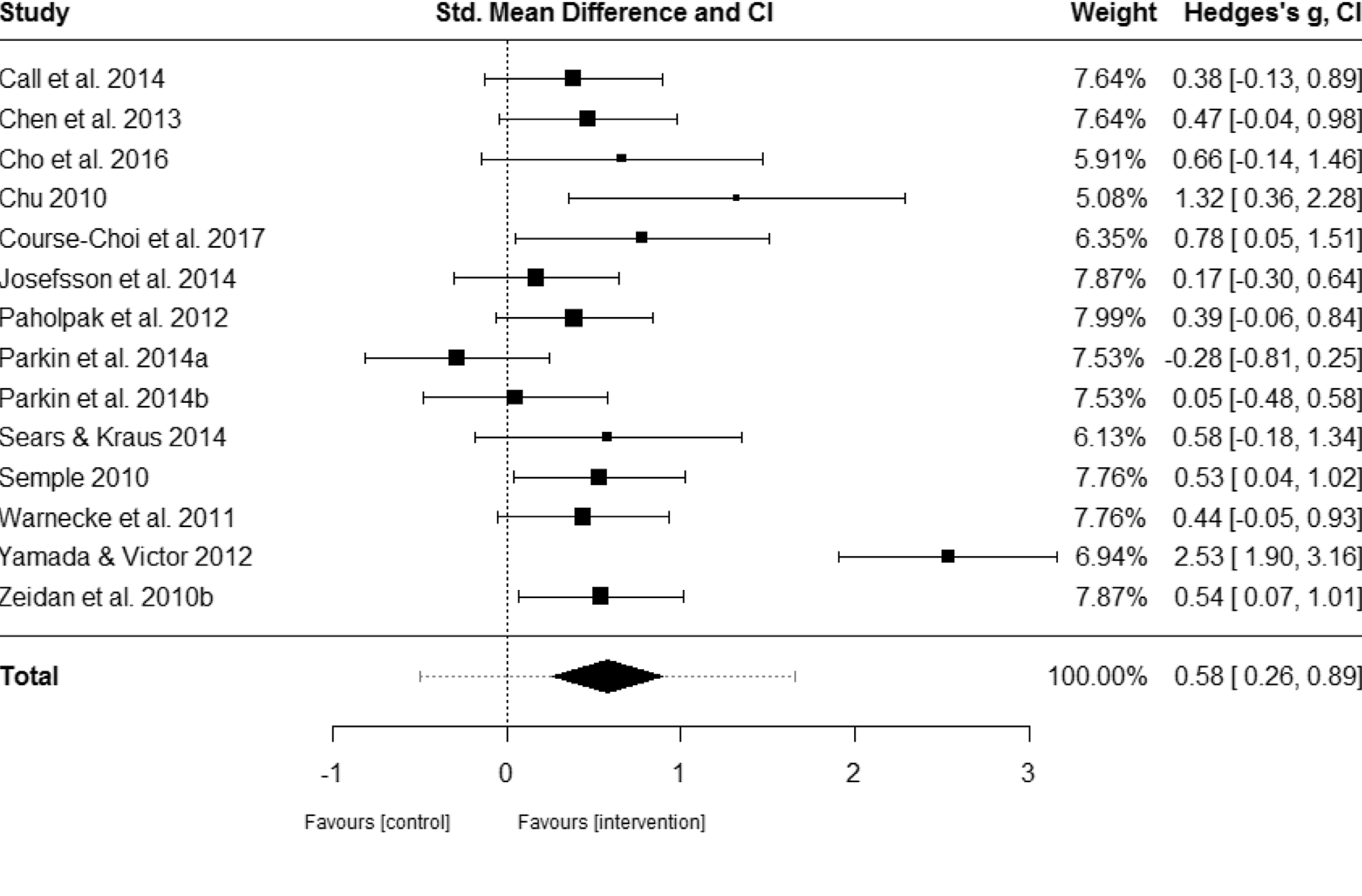
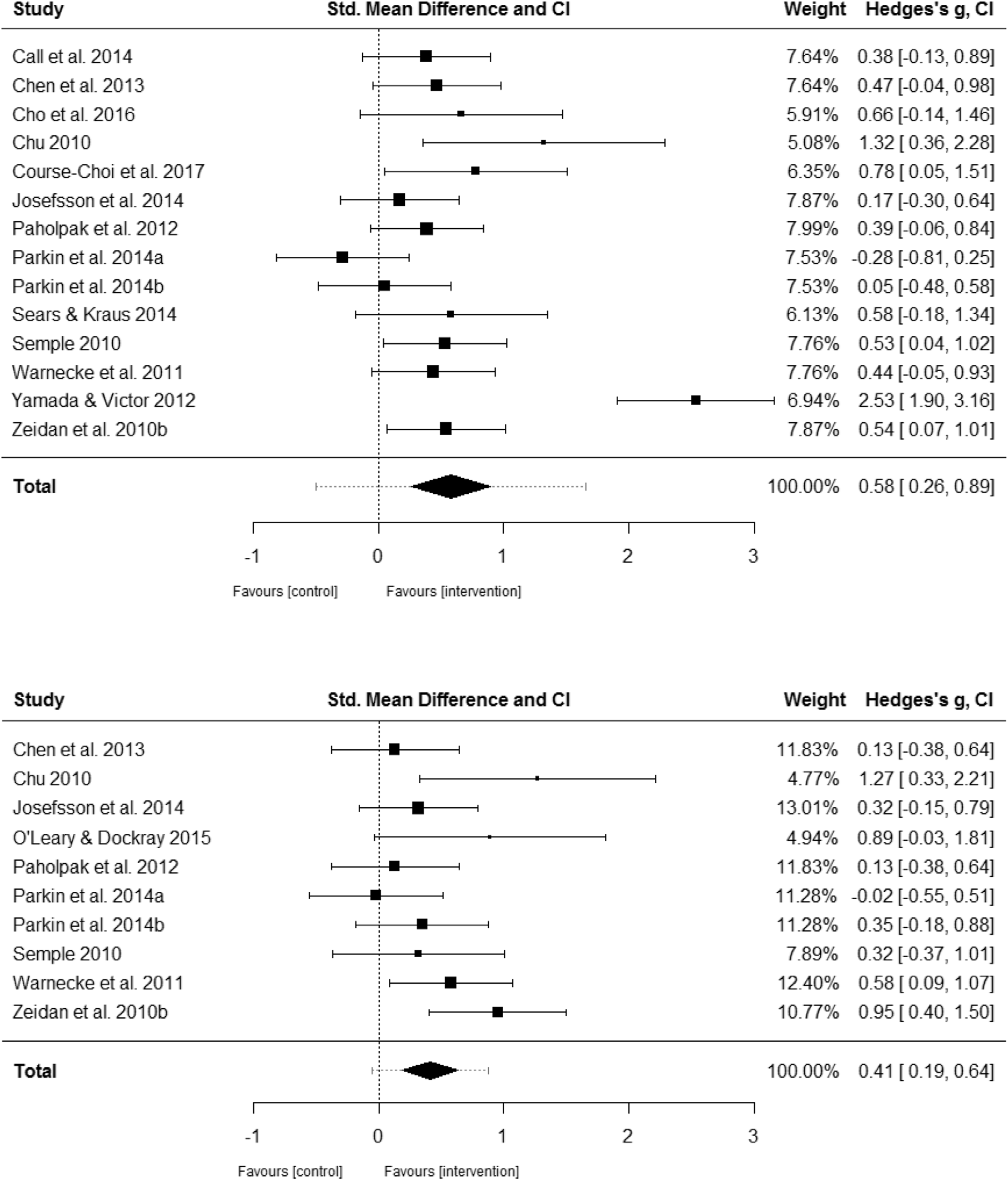
I’ve chosen the forest plot below from a recent meta-analysis published by Blanck et al. (2018). Interestingly, they examined the effect of stand-alone mindfulness exercises (SAMs) on depressive and anxiety symptoms rather than a therapeutic modality incorporating mindfulness. There’s been a substantial amount of interest in mindfulness-based interventions in the treatment of psychopathology and in generally for supporting positive well-being. Just simply google mindfulness research decades for images and you’ll find some notable charts showing significant growth in scientific studies published on mindfulness.
Nonetheless, here’s the published forest plot from that study, respectively, measuring effect on anxiety and depressive symptoms. The forest plot is a nice way to summarise estimated results from multiple independent studies. In this example, we can see that standalone mindfulness exercises have a significant effect on anxiety and depressive symptoms when compared to controls.
Figure 1: Forest plot of effect sizes of SAMs on anxiety and depressive symptoms. Adapted from Blanck et al. (2018).
Um, meta analysis?
Not being a statistician, by trade, compels me to figure out the basics of any statistical technique. Basics first right?
So, a meta-analysis is a statistical method for combining the results of a specified outcome from multiple scientific studies. The aim is to estimate the overall effect within a particular area of research. Essentially, the quantitative results from a meta-analysis is used to summarise a body of research (Egger & Smith, 1997). For example, there may be multiple independent studies undertaken on the effectiveness of Cognitive Behaviour Therapy (CBT) for depression. A meta-analysis could be completed to provide a quantitative review to consolidate the outcomes of CBT. The studies could be summarised by on the outcome measures used.
I’m going to use the meta-analysis published by Blanck et al. (2018) to practice how to replicate a meta-analysis. Plus, it was an interesting review on mindfulness-based exercises. Here’s the list of included studies that were used in the meta-analysis on anxiety symptoms (all studies are listed in the reference list):
Call, Miron, & Orcutt (2014); Chen, Yang, Wang, & Zhang (2013); Cho, Ryu, Noh, & Lee (2016); Chu (2010); Course-Choi, Saville, & Derakshan (2017); Josefsson, Lindwall, & Broberg (2014); Paholpak et al. (2012); Parkin et al. (2014); Sears & Kraus (2009); Semple (2010); Warnecke, Quinn, Ogden, Towle, & Nelson (2011); Yamada & Victor (2012); Zeidan, Johnson, Gordon, & Goolkasian (2010)
Collating all the statistics
It’s tedious but I went through all 14 studies included for the summary on anxiety symptoms and recorded the necessary statistics in Excel. Here’s there the data set from Excel that contains both all 14 studies with the Hedge’s $g$ statistic reported from Blanck et al. (2018) with the studies’ reported treatment group and control group mean scores and standard deviations.
# before reading data, we need to create a function for Cohen's d
# Blanck et al. (2018) used a controlled pre/post effect size calculation
# smd = standardised mean difference

# read in Excel studies data file
anxiety_studies_df <- readxl::read_excel("./data/replicating-meta-analysis-studies.xlsx",
                                         col_names = TRUE,
                                         sheet = "anxiety_es")

# take a look at the data
tibble::glimpse(anxiety_studies_df)
## Rows: 20
## Columns: 22
## $ study_name           <chr> "Call et al. (2014)", "Call et al. (2014)", "C...
## $ treatment_cond       <chr> "Body Scan", "Body Scan", "Meditation", "Mindf...
## $ control              <chr> "Waiting List", "Hatha Yoga", "No Intervention...
## $ inactive_control_ind <chr> "Y", "N", "Y", "Y", "N", "Y", "Y", "Y", "Y", "...
## $ outcome_measure      <chr> "DASS-21 - Anxiety", "DASS-21 - Anxiety", "SAS...
## $ notes                <chr> NA, NA, NA, NA, NA, NA, NA, NA, "This study di...
## $ year                 <dbl> 2014, 2014, 2013, 2016, 2016, 2010, 2017, 2014...
## $ blanck_hedge_g       <dbl> 0.38, 0.38, 0.47, 0.66, 0.66, 1.32, 0.78, 0.17...
## $ treatment_n          <dbl> 27, 29, 30, 12, 12, 10, 15, 38, 30, 20, 20, 20...
## $ treatment_pre        <dbl> 1.47, 1.88, 46.60, 49.75, 50.58, 1.04, 40.67, ...
## $ treatment_pre_sd     <dbl> 0.48, 0.73, 11.60, 5.71, 6.26, 0.90, 10.02, 4....
## $ treatment_post       <dbl> 1.34, 1.41, 41.40, 38.58, 41.17, 0.33, 35.00, ...
## $ treatment_post_sd    <dbl> 0.43, 0.42, 10.40, 10.04, 8.94, 0.34, 8.30, 3....
## $ treatment_sd_diff    <dbl> -0.05, -0.31, -1.20, 4.33, 2.68, -0.56, -1.72,...
## $ treatment_diff       <dbl> -0.13, -0.47, -5.20, -11.17, -9.41, -0.71, -5....
## $ control_n            <dbl> 35, 35, 30, 12, 12, 10, 15, 30, 28, 20, 20, 20...
## $ control_pre          <dbl> 1.66, 1.66, 46.20, 47.92, 47.92, 1.51, 35.73, ...
## $ control_pre_sd       <dbl> 0.56, 0.56, 11.50, 7.74, 7.74, 0.92, 10.24, 4....
## $ control_post         <dbl> 1.78, 1.78, 46.30, 43.33, 43.33, 1.63, 37.47, ...
## $ control_post_sd      <dbl> 0.77, 0.77, 11.80, 8.49, 8.49, 0.80, 10.09, 3....
## $ control_sd_diff      <dbl> 0.21, 0.21, 0.30, 0.75, 0.75, -0.12, -0.15, -0...
## $ control_diff         <dbl> 0.12, 0.12, 0.10, -4.59, -4.59, 0.12, 1.74, -1...

# take a different look at the data
head(anxiety_studies_df, 5) %>%
  knitr::kable() %>%
  kableExtra::kable_styling(c("bordered", "condensed"), full_width = T, position = "l") %>%
scroll_box(width = "100%", height = "400px")| study_name | treatment_cond | control | inactive_control_ind | outcome_measure | notes | year | blanck_hedge_g | treatment_n | treatment_pre | treatment_pre_sd | treatment_post | treatment_post_sd | treatment_sd_diff | treatment_diff | control_n | control_pre | control_pre_sd | control_post | control_post_sd | control_sd_diff | control_diff |
|---|---|---|---|---|---|---|---|---|---|---|---|---|---|---|---|---|---|---|---|---|---|
| Call et al. (2014) | Body Scan | Waiting List | Y | DASS-21 - Anxiety | NA | 2014 | 0.38 | 27 | 1.47 | 0.48 | 1.34 | 0.43 | -0.05 | -0.13 | 35 | 1.66 | 0.56 | 1.78 | 0.77 | 0.21 | 0.12 |
| Call et al. (2014) | Body Scan | Hatha Yoga | N | DASS-21 - Anxiety | NA | 2014 | 0.38 | 29 | 1.88 | 0.73 | 1.41 | 0.42 | -0.31 | -0.47 | 35 | 1.66 | 0.56 | 1.78 | 0.77 | 0.21 | 0.12 |
| Chen et al. (2013) | Meditation | No Intervention | Y | SAS | NA | 2013 | 0.47 | 30 | 46.60 | 11.60 | 41.40 | 10.40 | -1.20 | -5.20 | 30 | 46.20 | 11.50 | 46.30 | 11.80 | 0.30 | 0.10 |
| Cho et al. (2016) | Mindful Breathing Practice | No Intervention | Y | Revised Test Anxiety | NA | 2016 | 0.66 | 12 | 49.75 | 5.71 | 38.58 | 10.04 | 4.33 | -11.17 | 12 | 47.92 | 7.74 | 43.33 | 8.49 | 0.75 | -4.59 |
| Cho et al. (2016) | Mindful Breathing Practice | Cognitive Reappraisal Practice | N | Revised Test Anxiety | NA | 2016 | 0.66 | 12 | 50.58 | 6.26 | 41.17 | 8.94 | 2.68 | -9.41 | 12 | 47.92 | 7.74 | 43.33 | 8.49 | 0.75 | -4.59 |
Great. So we have the data stored and ready for further analysis but now we need to use those statistics to calculate the effect size. Luckily, Blanck et al. (2018) have provided the equation in their paper on how they estimate Cohen’s $d$ and Hedge’s h. Makes my life a lot easier!
We could use a standard function to calculate the effect size, for example, esc_mean_gain() from the esc package. I’ll compare the differences in the estimates later on using a user-defined function and a package provided function.
Computing an effect size
Adopting the equations
Time to create a function for both the Cohen’s $d$ equation and Hedge’s $g$ equations in Blanck et al. (2018). Both of these equations are used to estimate the controlled pre/post effect size. First off, I’m going to define a function that will take those parameters of the equation and calculate an Cohen’s $d$. Also, I’m going to define a separate function that will convert Cohen’s $d$ to Hedge’s $g$. Respectively, we’ll call the function cohen_d_calc() and convert_d_g(). For reference, here is the equation for calculating the pre/post controlled effect size (Blanck et al., 2018):
$$d=\frac{\Delta_1-\Delta_2}{\sqrt{\frac{(n_1-1)S_1^2+(n_2-1)S_2^2}{n_1+n_2-2}}}$$
where $\Delta_1$ refers to the difference between the pre- and post-treatment mean score/value and $\Delta_2$ refers to the difference between the post- and post-control mean score/value. $S_1$ and $S_2$ refers, respectively, to the standard deviations of the treatment and control post scores. $n_1$ and $n_2$ refers to the sample size of, respectively, the treatment and control groups for complete pre/post observations.
There are slight variations of the above equation reported in Morris (2008) (see equations [8-10]) and Lakens (2013) (see equation [1]). The mathematical interpretation of these equations is far beyond my knowledge so I’m going to stay clear of that.
The equation for converting Cohen’s $d$ into Hedge’s $g$ is described below:
$$g=d*(1-\frac{3}{4df-1})$$
where $d$ is the estimated pre/post controlled effect size according to Cohen’s $d$ and $df$ refers to the degrees of freedom. Let’s now put this into functions in R so that we can estimate the effect sizes accordingly for each study later on.
# create function for calculating Cohen's d as per the Blanck et al. (2018) provided equation
cohen_d_calc <- function(

  # specify all the arguments, i.e. pre/post means, pre/post sd etc
  treatment_pre_mean,
  treatment_post_mean,
  treatment_post_sd,
  control_pre_mean,
  control_post_mean,
  control_post_sd,
  treatment_n,
  control_n) {

  # numerator: mean differences for pre MINUS mean differences for post
  ( ( treatment_pre_mean - treatment_post_mean ) - ( control_pre_mean - control_post_mean ) ) /

    # denominator: pooled standard deviation
    (
      sqrt
      (
        # numerator
        ( ( ( treatment_n - 1 ) * ( treatment_post_sd ^ 2 ) ) + ( ( control_n - 1 ) * ( control_post_sd ^ 2 ) ) ) /

          # denominator
          ( treatment_n + control_n - 2 )
      )
    )
}

# conversion from Cohen's d to Hedge's g
convert_d_g <- function(d, treatment_n, control_n) {

  # Cohen's d multipled by conversion factor
  d * ( 1 - ( 3 / ( ( 4 * ( treatment_n + control_n ) ) ) ) )

}

# create a function for pooled standard deviations
pooled_sd <- function(

  # specify all the arguments, i.e. pre/post means, pre/post sd etc
  treatment_post_sd,
  control_post_sd,
  treatment_n,
  control_n

) {

  sqrt
  (
    # numerator
    ( ( ( treatment_n - 1 ) * ( treatment_post_sd ^ 2 ) ) + ( ( control_n - 1 ) * ( control_post_sd ^ 2 ) ) ) /

      # denominator
      ( treatment_n + control_n - 2 )
  )
}
We have these equations in the form of functions but does it actually work? Let’s test it out on the first study reported in the forest plot for anxiety symptoms, i.e. Call et al. (2014).
# calculate Cohen's d first
call_d <- cohen_d_calc(treatment_pre_mean = 1.47,
                       treatment_post_mean = 1.34,
                       treatment_post_sd = 0.43,
                       control_pre_mean = 1.66,
                       control_post_mean = 1.78,
                       control_post_sd = 0.77,
                       treatment_n = 27,
                       control_n = 35)
call_d
## [1] 0.387562

# then convert to Hedge's g
call_h <- convert_d_g(d = call_d,
                      treatment_n = 27,
                      control_n = 35)
round(call_h, 2)
## [1] 0.38

# exact result as per Blanck et al. (2018) reported result
# h = 0.38
Okay, this is looking promising as the Hedge’s $g$ value I’ve calculated is the same as the one published by Call et al. (2014). The real test will be to apply this function to the remaining studies.
Applying the function to all studies
Remember that we have imported all the statistics from each studies in the Excel data file. It’s just then a matter of creating a new column that (1) calculates Cohen’s $d$; and then (2) converts $d$ into Hedge’s $g$. We’ll filter the data frame so that only studies with an inactive control comparison are included as per the filter(inactive_control_ind == "Y") line. From that, we use our function for calculating $d$, i.e. the cohen_d_calc() function followed by converting it into $g$. Let’s go ahead and create a few columns estimating the effect sizes using our custom functions.
# create a new variable that provides both d and g
anxiety_studies_eff_df <- anxiety_studies_df %>%
  filter(inactive_control_ind == "Y") %>%
  mutate(cohen_d_val = cohen_d_calc(treatment_pre_mean = treatment_pre,
                                    treatment_post_mean = treatment_post,
                                    treatment_post_sd = treatment_post_sd,
                                    control_pre_mean = control_pre,
                                    control_post_mean = control_post,
                                    control_post_sd = control_post_sd,
                                    treatment_n = treatment_n,
                                    control_n = control_n),
         study_pooled_sd = pooled_sd(treatment_post_sd = treatment_post_sd,
                                     control_post_sd = control_post_sd,
                                     treatment_n = treatment_n,
                                     control_n = control_n)) %>%
  mutate(hedge_g_val = convert_d_g(cohen_d_val, treatment_n, control_n),
         hedge_g_rounded = round(hedge_g_val, 2)) %>%
  dplyr::select(study_name, year, blanck_hedge_g, hedge_g_rounded, cohen_d_val, hedge_g_val, everything())
We should now have a data frame that contains the published effect sizes from Blanck et al. (2018) and the estimated effect sizes from our functions. Take a look at it below:
# take a different look at the data
anxiety_studies_eff_df %>%
  knitr::kable() %>%
  kableExtra::kable_styling(c("bordered", "condensed"), full_width = T, position = "l") %>%
scroll_box(width = "100%", height = "400px")| study_name | year | blanck_hedge_g | hedge_g_rounded | cohen_d_val | hedge_g_val | treatment_cond | control | inactive_control_ind | outcome_measure | notes | treatment_n | treatment_pre | treatment_pre_sd | treatment_post | treatment_post_sd | treatment_sd_diff | treatment_diff | control_n | control_pre | control_pre_sd | control_post | control_post_sd | control_sd_diff | control_diff | study_pooled_sd |
|---|---|---|---|---|---|---|---|---|---|---|---|---|---|---|---|---|---|---|---|---|---|---|---|---|---|
| Call et al. (2014) | 2014 | 0.38 | 0.38 | 0.3875620 | 0.3828737 | Body Scan | Waiting List | Y | DASS-21 - Anxiety | NA | 27 | 1.47 | 0.48 | 1.34 | 0.43 | -0.05 | -0.13 | 35 | 1.66 | 0.56 | 1.78 | 0.77 | 0.21 | 0.12 | 0.416100 |
| Chen et al. (2013) | 2013 | 0.47 | 0.47 | 0.4765308 | 0.4705742 | Meditation | No Intervention | Y | SAS | NA | 30 | 46.60 | 11.60 | 41.40 | 10.40 | -1.20 | -5.20 | 30 | 46.20 | 11.50 | 46.30 | 11.80 | 0.30 | 0.10 | 123.700000 |
| Cho et al. (2016) | 2016 | 0.66 | 0.69 | 0.7077280 | 0.6856115 | Mindful Breathing Practice | No Intervention | Y | Revised Test Anxiety | NA | 12 | 49.75 | 5.71 | 38.58 | 10.04 | 4.33 | -11.17 | 12 | 47.92 | 7.74 | 43.33 | 8.49 | 0.75 | -4.59 | 86.440850 |
| Chu (2010) | 2010 | 1.32 | 1.30 | 1.3503524 | 1.2997142 | Meditation | No Intervention | Y | GHQ-28 - Anxiety and Insomnia | NA | 10 | 1.04 | 0.90 | 0.33 | 0.34 | -0.56 | -0.71 | 10 | 1.51 | 0.92 | 1.63 | 0.80 | -0.12 | 0.12 | 0.377800 |
| Course-Choi et al. (2017) | 2017 | 0.78 | 0.78 | 0.8020822 | 0.7820301 | Mindfulness | No Intervention | Y | STAI-S - Anxiety | NA | 15 | 40.67 | 10.02 | 35.00 | 8.30 | -1.72 | -5.67 | 15 | 35.73 | 10.24 | 37.47 | 10.09 | -0.15 | 1.74 | 85.349050 |
| Josefsson et al. (2014) | 2014 | 0.17 | 0.17 | 0.1707681 | 0.1688846 | Mindfulness | Waiting List | Y | HAD-A | NA | 38 | 8.22 | 4.50 | 5.92 | 3.60 | -0.90 | -2.30 | 30 | 8.60 | 4.40 | 6.93 | 3.80 | -0.60 | -1.67 | 13.610303 |
| Paholpak et al. (2012) | 2012 | 0.39 | NA | NA | NA | Meditation | No Intervention | Y | SCL-90-Anxiety | This study didn’t provide Mean and SDs | 30 | NA | NA | NA | NA | NA | NA | 28 | NA | NA | NA | NA | NA | NA | NA |
| Parkin et al. (2014a) | 2014 | -0.28 | -0.18 | -0.1856234 | -0.1821430 | Body Scan | No Intervention | Y | STAI-T | Both Body Scan and Sound Scan are meditation techniques. | 20 | 28.45 | 8.01 | 28.45 | 6.71 | -1.30 | 0.00 | 20 | 37.25 | 9.57 | 35.45 | 11.96 | 2.39 | -1.80 | 94.032850 |
| Parkin et al. (2014a) | 2014 | -0.28 | -0.38 | -0.3896593 | -0.3823532 | Sound Scan | No Intervention | Y | STAI-T | Both Body Scan and Sound Scan are meditation techniques. | 20 | 27.40 | 4.31 | 29.10 | 4.28 | -0.03 | 1.70 | 20 | 37.25 | 9.57 | 35.45 | 11.96 | 2.39 | -1.80 | 80.680000 |
| Parkin et al. (2014b) | 2014 | 0.05 | 0.05 | 0.0468202 | 0.0459423 | Body Scan | No Intervention | Y | STAI-T | Both Body Scan and Sound Scan are meditation techniques. | 20 | 37.16 | 7.73 | 35.95 | 9.03 | 1.30 | -1.21 | 20 | 35.95 | 10.10 | 35.20 | 10.56 | 0.46 | -0.75 | 96.527250 |
| Parkin et al. (2014b) | 2014 | 0.05 | 0.06 | 0.0599431 | 0.0588192 | Sound Scan | No Intervention | Y | STAI-T | Both Body Scan and Sound Scan are meditation techniques. | 20 | 37.85 | 11.86 | 36.45 | 11.12 | -0.74 | -1.40 | 20 | 35.95 | 10.10 | 35.20 | 10.56 | 0.46 | -0.75 | 117.584000 |
| Sears & Kraus (2009) | 2009 | 0.58 | 0.58 | 0.5969620 | 0.5815233 | Brief Meditation Focused on Attention | No Intervention | Y | BAI | There are multiple mindfulness treatment groups. | 19 | 8.19 | 6.52 | 7.90 | 5.93 | -0.59 | -0.29 | 10 | 10.49 | 8.39 | 14.91 | 10.79 | 2.40 | 4.42 | 62.251300 |
| Semple (2010) | 2010 | 0.53 | NA | NA | NA | Body Scan | Waiting List | Y | STAI | NA | 15 | NA | NA | NA | NA | NA | NA | 16 | NA | NA | NA | NA | NA | NA | NA |
| Warnecke et al. (2011) | 2011 | 0.44 | NA | NA | NA | Meditation | Waiting List | Y | DASS-21 - Anxiety | NA | 31 | 8.10 | 6.50 | NA | NA | NA | NA | 30 | NA | NA | NA | NA | NA | NA | NA |
| Yamada & Victor (2012) | 2012 | 2.53 | 3.22 | 3.2586721 | 3.2179387 | Meditation | No Intervention | Y | STAI-S | NA | 37 | 40.50 | 2.00 | 38.70 | 2.40 | 0.40 | -1.80 | 23 | 37.00 | 2.70 | 44.10 | 3.20 | 0.50 | 7.10 | 7.459310 |
| Yamada & Victor (2012) | 2012 | 2.53 | 1.85 | 1.8770438 | 1.8535807 | Meditation | No Intervention | Y | STAI-T | NA | 37 | 41.60 | 1.80 | 39.90 | 2.00 | 0.20 | -1.70 | 23 | 38.20 | 2.40 | 40.80 | 2.70 | 0.30 | 2.60 | 5.247931 |
| Zeidan et al. (2010b) | 2010 | 0.54 | 1.08 | 1.0941572 | 1.0792369 | Meditation | No Intervention | Y | STAI-S | NA | 29 | 40.93 | 8.47 | 29.28 | 6.72 | -1.75 | -11.65 | 26 | 35.19 | 10.47 | 32.32 | 9.27 | -1.20 | -2.87 | 64.391655 |
| Zeidan et al. (2010b) | 2010 | 0.54 | 1.08 | 1.0941572 | 1.0792369 | Meditation | No Intervention | Y | POMS - Tension/Anxiety | NA | 29 | 40.93 | 8.47 | 29.28 | 6.72 | -1.75 | -11.65 | 26 | 35.19 | 10.47 | 32.32 | 9.27 | -1.20 | -2.87 | 64.391655 |
However, I’m missing another required transformation. There are two studies which, in fact, used multiple treatment conditions and compared them against an inactive control group, i.e. Parkin et al. (2014) and Yamada & Victor (2012). We have estimated the effect size for these studies but have not combined these together to represent the study overall.
I’ve decided to calculate the weighted mean effect size for these studies which I assume is what the authors in Blanck et al. (2018, p. 28) similarly did:
If studies provided data for more than one eligible outcome measure of either anxiety or depression, we collapsed data to ensure independence of obtained ESs. In a similar vein, data was combined for studies using multiple, eligible treatment conditions (e.g., conditions employing different mindfulness exercises).
The equation for the weighted estimator can be found in Hedges (1983). Here it is below:
$$\overline{x}=\frac{\sum_{i=1}^{k}w_{i}g_{i}}{\sum_{i=1}^{k}w_{i}}$$
where $\overline{x}$ is the calculation for weighted mean effect size.
In our case, the weight $w_{i}$ refers to the total sample size for the given study$_{i}$ including both treatment and control groups. $g_{i}$ refers to the effect size estimated for the study$_{i}$. Okay, let’s take care of those studies by calculating the weighted mean effect size and then compare it against the reported effect sizes.
If effect sizes in studies could not be calculated, we’ll adopt Hedge’s $g$ reported from the meta-analysis. Furthermore, pretest and pottest scores were only reported for one of the two anxiety scales in Zeidan et al. (2010). Given the insufficient information, we will substitute our estimated $g$ value with the published value.
# calculate weighted mean effect size and compare with Blanck et al. (2018)
anxiety_wgt_eff_df <- anxiety_studies_eff_df %>%
  mutate(total_n = treatment_n + control_n,
         weight = total_n * hedge_g_val) %>%
  group_by(study_name) %>%
  summarise(weighted_g_val = round(sum(weight) / sum(total_n), 2)) %>%
  dplyr::left_join(x = .,
                   y = anxiety_studies_eff_df %>%
                     distinct(study_name, blanck_hedge_g, treatment_n, control_n),
                   by = "study_name") %>%
  mutate(weighted_g_val = ifelse(is.na(weighted_g_val) |
                                   study_name == "Zeidan et al. (2010b)", blanck_hedge_g, weighted_g_val))
anxiety_wgt_eff_df
## # A tibble: 14 x 5
##    study_name                weighted_g_val blanck_hedge_g treatment_n control_n
##    <chr>                              <dbl>          <dbl>       <dbl>     <dbl>
##  1 Call et al. (2014)                 0.38           0.38           27        35
##  2 Chen et al. (2013)                 0.47           0.47           30        30
##  3 Cho et al. (2016)                  0.69           0.66           12        12
##  4 Chu (2010)                         1.3            1.32           10        10
##  5 Course-Choi et al. (2017)          0.78           0.78           15        15
##  6 Josefsson et al. (2014)            0.17           0.17           38        30
##  7 Paholpak et al. (2012)             0.39           0.39           30        28
##  8 Parkin et al. (2014a)             -0.28          -0.28           20        20
##  9 Parkin et al. (2014b)              0.05           0.05           20        20
## 10 Sears & Kraus (2009)               0.580          0.580          19        10
## 11 Semple (2010)                      0.53           0.53           15        16
## 12 Warnecke et al. (2011)             0.44           0.44           31        30
## 13 Yamada & Victor (2012)             2.54           2.53           37        23
## 14 Zeidan et al. (2010b)              0.54           0.54           29        26
It’s coming along well. There’s some small differences that we’ll tolerate for now (especially given that this is new to me). So, we have the effect sizes. What are now missing? Bloody sampling variances for the studies.
Pretest-posttest correlations
Unfortunately, none of the studies included for the meta-analysis on anxiety symptoms included correlations between pretest and posttest results. The methodology also does include any information on how this correlation coefficient was determined. These are required in order to calculated the sampling variance vi in the metafor::rma package.
A previous meta-analysis on mindfulness and its effect on anxiety and depression has encountered the same issue (Hofmann, Sawyer, Witt, & Oh, 2010; Hofmann, Wu, & Boettcher, 2014). To address this, the authors used a conservative estimation of $r$ = .7 in accordance to Rosenthal (1986)’s recommendation. Similarly, I will use .7 and test out the forest plot.
Seeing the forest for the trees
Before I can replicate the forest plot, I need to set the pretest and posttest correlation coefficient ri. Since we have estimated the effect sizes already, we can use the approach in Morris (2008) to determine the sampling variance vi which is required to run a random-effects model. Yes, very confusing. See Viechtbauer (n.d.) as the webpage contains more information on the R syntax for using pooled standard deviations to calculating the sampling variance using the approach described in Morris (2008).
So, let’s therefore use $r=.7$ for the pretest and posttest correlation and feed it into the calculation for sampling variance as per vi in the metafor::rma() function.
# use .7 for pre/post correlation to calculate the sampling variance
# see http://www.metafor-project.org/doku.php/analyses:morris2008 for more information
r = 0.7
anxiety_ri_vi_df <- anxiety_wgt_eff_df %>%
  mutate(ri = r,
         vi = 2*(1-ri) *
           (1/treatment_n + 1/control_n) +
           weighted_g_val^2 / (2*(treatment_n + control_n)))
anxiety_ri_vi_df
## # A tibble: 14 x 7
##    study_name   weighted_g_val blanck_hedge_g treatment_n control_n    ri     vi
##    <chr>                 <dbl>          <dbl>       <dbl>     <dbl> <dbl>  <dbl>
##  1 Call et al.~          0.38           0.38           27        35   0.7 0.0405
##  2 Chen et al.~          0.47           0.47           30        30   0.7 0.0418
##  3 Cho et al. ~          0.69           0.66           12        12   0.7 0.110
##  4 Chu (2010)            1.3            1.32           10        10   0.7 0.162
##  5 Course-Choi~          0.78           0.78           15        15   0.7 0.0901
##  6 Josefsson e~          0.17           0.17           38        30   0.7 0.0360
##  7 Paholpak et~          0.39           0.39           30        28   0.7 0.0427
##  8 Parkin et a~         -0.28          -0.28           20        20   0.7 0.0610
##  9 Parkin et a~          0.05           0.05           20        20   0.7 0.0600
## 10 Sears & Kra~          0.580          0.580          19        10   0.7 0.0974
## 11 Semple (201~          0.53           0.53           15        16   0.7 0.0820
## 12 Warnecke et~          0.44           0.44           31        30   0.7 0.0409
## 13 Yamada & Vi~          2.54           2.53           37        23   0.7 0.0961
## 14 Zeidan et a~          0.54           0.54           29        26   0.7 0.0464
After all that trouble, we finally have the complete set of statistics to plug into the random effects model function. At this point, I’m going to use the metafor::rma() function which will aggregate all the effect sizes to produce a summary effect size of SAMs on anxiety symptoms. Good news is that we know that Blanck et al. (2018) used the inverse variance random effects model by DerSimonian & Laird (1986). You can choose this model by specifying method = "DL" in the rma() function. See below.
# random effects model with r = .7
# fit the re model
res <- metafor::rma(data = anxiety_ri_vi_df,
                    yi = weighted_g_val, # effect size
                    vi = vi, # sampling
                    method = "DL",
                    slab = study_name)
res
##
## Random-Effects Model (k = 14; tau^2 estimator: DL)
##
## tau^2 (estimated amount of total heterogeneity): 0.2412 (SE = 0.1238)
## tau (square root of estimated tau^2 value):      0.4911
## I^2 (total heterogeneity / total variability):   80.19%
## H^2 (total variability / sampling variability):  5.05
##
## Test for Heterogeneity:
## Q(df = 13) = 65.6255, p-val < .0001
##
## Model Results:
##
## estimate      se    zval    pval   ci.lb   ci.ub
##   0.5771  0.1487  3.8811  0.0001  0.2857  0.8686  ***
##
## ---
## Signif. codes:  0 '***' 0.001 '**' 0.01 '*' 0.05 '.' 0.1 ' ' 1

# finally plot the damn thing!
metafor::forest(res,
                showweights = TRUE,
                xlim = c(-4,6),
                xlab = "Effect Size (Hedge's g)",
                # digits = c(2,3p),
                mlab = "Total",
                cex = 0.75,
                cex.lab = 0.75)

# switch to bold
par(font = 2)

# add column headings to the plot
text(x = -3, y = 17, labels = "Author(s) and Year", cex = 0.75, pos = 1)
text(x = 0, y = 17, labels = "Std. Mean Difference and CI", cex = 0.75, pos = 1)
text(x = 4, y = 17, labels = "Weights", cex = 0.75, pos = 1)
text(x = 5.1, y = 17, labels = "Hedge's g, CI", cex = 0.75, pos = 1)

# add x axis label
text(x = -1, y = -2, labels = "Favours [control]", cex = 0.75, pos=1)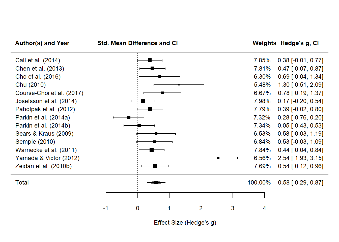
Finally, a plot!
However, the confidence intervals for each study’s effect sizes are far off from the ones reported in the meta-analysis. With some trial and error, I assumed that $r=.5$ might be more conservative than the value adopted from Rosenthal (1986). There’s no information about what correlation coefficient was used in Blanck et al. (2018).
All in one go:
# use .5 for pre/post correlation to calculate the sampling variance
# see http://www.metafor-project.org/doku.php/analyses:morris2008 for more information
r = 0.5
anxiety_ri_vi_df <- anxiety_wgt_eff_df %>%
  mutate(ri = r,
         vi = 2*(1-ri) *
           (1/treatment_n + 1/control_n) +
           weighted_g_val^2 / (2*(treatment_n + control_n)))
anxiety_ri_vi_df
## # A tibble: 14 x 7
##    study_name   weighted_g_val blanck_hedge_g treatment_n control_n    ri     vi
##    <chr>                 <dbl>          <dbl>       <dbl>     <dbl> <dbl>  <dbl>
##  1 Call et al.~          0.38           0.38           27        35   0.5 0.0668
##  2 Chen et al.~          0.47           0.47           30        30   0.5 0.0685
##  3 Cho et al. ~          0.69           0.66           12        12   0.5 0.177
##  4 Chu (2010)            1.3            1.32           10        10   0.5 0.242
##  5 Course-Choi~          0.78           0.78           15        15   0.5 0.143
##  6 Josefsson e~          0.17           0.17           38        30   0.5 0.0599
##  7 Paholpak et~          0.39           0.39           30        28   0.5 0.0704
##  8 Parkin et a~         -0.28          -0.28           20        20   0.5 0.101
##  9 Parkin et a~          0.05           0.05           20        20   0.5 0.100
## 10 Sears & Kra~          0.580          0.580          19        10   0.5 0.158
## 11 Semple (201~          0.53           0.53           15        16   0.5 0.134
## 12 Warnecke et~          0.44           0.44           31        30   0.5 0.0672
## 13 Yamada & Vi~          2.54           2.53           37        23   0.5 0.124
## 14 Zeidan et a~          0.54           0.54           29        26   0.5 0.0756

# random effects model with r = .5
# fit the re model
res <- metafor::rma(data = anxiety_ri_vi_df,
                    yi = weighted_g_val, # effect size
                    vi = vi, # sampling
                    method = "DL",
                    slab = study_name)
res
##
## Random-Effects Model (k = 14; tau^2 estimator: DL)
##
## tau^2 (estimated amount of total heterogeneity): 0.2536 (SE = 0.1422)
## tau (square root of estimated tau^2 value):      0.5036
## I^2 (total heterogeneity / total variability):   72.49%
## H^2 (total variability / sampling variability):  3.64
##
## Test for Heterogeneity:
## Q(df = 13) = 47.2558, p-val < .0001
##
## Model Results:
##
## estimate      se    zval    pval   ci.lb   ci.ub
##   0.5781  0.1605  3.6020  0.0003  0.2635  0.8927  ***
##
## ---
## Signif. codes:  0 '***' 0.001 '**' 0.01 '*' 0.05 '.' 0.1 ' ' 1

# finally plot the damn thing!
metafor::forest(res,
                showweights = TRUE,
                xlim = c(-4,6),
                xlab = "Effect Size (Hedge's g)",
                # digits = c(2,3p),
                mlab = "Total",
                cex = 0.75,
                cex.lab = 0.75)

# switch to bold
par(font = 2)

# add column headings to the plot
text(x = -3, y = 17, labels = "Author(s) and Year", cex = 0.75, pos = 1)
text(x = 0, y = 17, labels = "Std. Mean Difference and CI", cex = 0.75, pos = 1)
text(x = 4, y = 17, labels = "Weights", cex = 0.75, pos = 1)
text(x = 5.1, y = 17, labels = "Hedge's g, CI", cex = 0.75, pos = 1)

# add x axis label
text(x = -1, y = -2, labels = "Favours [control]", cex = 0.75, pos=1)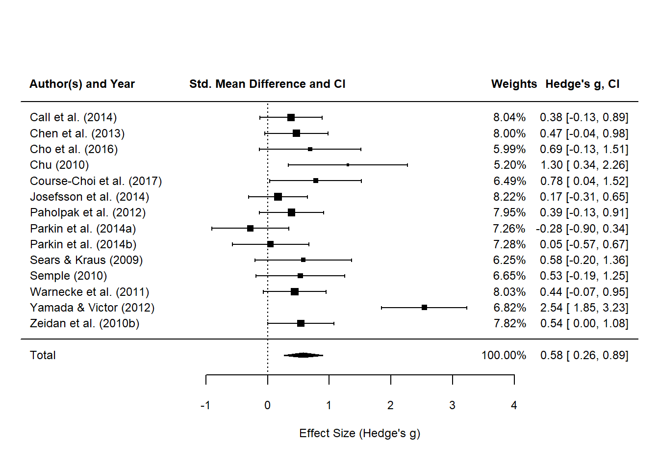
… let’s serve up the original plot from the meta-analysis to compare.

The Hedge’s $g$ values come quite close to the results reported in the meta-analysis for Blanck et al. (2018). The random effects model yielded the same summary effect size of SAMs (and confidence intervals) on anxiety symptoms as per the forest plot in Blanck et al. (2018), i.e. $SMD=0.58$. However, the weights reported by our model do not match the ones published in the article. I admimttedly can’t explain this at this stage.
Nonetheless, I think this is an OK attempt at the basics of completing a meta-analysis. This does not cover all the processes involved in running a meta-analysis and I would recommend a relevant and recent article by Shim & Kim (2019) that provide additional examples on sorting out intervention meta-analyses in R. The authors also provide a nifty diagram on the essentials of the meta-analytic process.
I might write another post on how to use the packages directly to perform the manual effect size calculations automatically.
Key takeaways
Well, firstly, brief standalone mindfulness practice appears to have a positive effect on reducing anxiety symptoms. This includes a variety of exercises (and modes) such as body scans, breathing meditation etc. Also, it’s nice to see similar efficacy in Blanck et al. (2018) and Hofmann et al. (2010) (a meta-analysis on mindfulness-based therapy rather than standalone mindfulness exercises). This raises questions about when it is suitable (and perhaps more cost effective) to administer brief mindfulness exercises without other therapeutic components and for which group(s).
Not all studies will report the required statistics to use as your input into effect size calculations. This makes the meta-analytical process challenging especially when you need key statistics such as pretest and posttest mean scores and standard deviations and pre/post correlations. Some studies may also include only figures without the associated values for the data points making your life even more difficult.
One counterintuitive takeaway is that manually calculating the effect sizes was more informative than using pre-defined functions in packages such as
esc,effsize,psych,meta,metafor. These packages are absolutely powerful but I found it beneficial in getting down to the nuts and bolts of manually calculating the effect sizes which the aforementioned packages can do anyway. That’s just me.I do not envy statisticians!
References
Blanck, P., Perleth, S., Heidenreich, T., Kröger, P., Ditzen, B., Bents, H., & Mander, J. (2018). Effects of mindfulness exercises as stand-alone intervention on symptoms of anxiety and depression: Systematic review and meta-analysis. Behaviour Research and Therapy, 102, 25–35.
Call, D., Miron, L., & Orcutt, H. (2014). Effectiveness of brief mindfulness techniques in reducing symptoms of anxiety and stress. Mindfulness, 5(6), 658–668.
Chen, Y., Yang, X., Wang, L., & Zhang, X. (2013). A randomized controlled trial of the effects of brief mindfulness meditation on anxiety symptoms and systolic blood pressure in chinese nursing students. Nurse Education Today, 33(10), 1166–1172.
Cho, H., Ryu, S., Noh, J., & Lee, J. (2016). The effectiveness of daily mindful breathing practices on test anxiety of students. PloS One, 11(10), e0164822.
Chu, L.-C. (2010). The benefits of meditation vis-à-vis emotional intelligence, perceived stress and negative mental health. Stress and Health: Journal of the International Society for the Investigation of Stress, 26(2), 169–180.
Course-Choi, J., Saville, H., & Derakshan, N. (2017). The effects of adaptive working memory training and mindfulness meditation training on processing efficiency and worry in high worriers. Behaviour Research and Therapy, 89, 1–13.
DerSimonian, R., & Laird, N. (1986). Meta-analysis in clinical trials. Controlled Clinical Trials, 7(3), 177–188.
Egger, M., & Smith, G. D. (1997). Meta-analysis: Potentials and promise. Bmj, 315(7119), 1371–1374.
Hedges, L. V. (1983). A random effects model for effect sizes. Psychological Bulletin, 93(2), 388.
Hofmann, S. G., Sawyer, A. T., Witt, A. A., & Oh, D. (2010). The effect of mindfulness-based therapy on anxiety and depression: A meta-analytic review. Journal of Consulting and Clinical Psychology, 78(2), 169.
Hofmann, S. G., Wu, J. Q., & Boettcher, H. (2014). Effect of cognitive-behavioral therapy for anxiety disorders on quality of life: A meta-analysis. Journal of Consulting and Clinical Psychology, 82(3), 375.
Josefsson, T., Lindwall, M., & Broberg, A. G. (2014). The effects of a short-term mindfulness based intervention on self-reported mindfulness, decentering, executive attention, psychological health, and coping style: Examining unique mindfulness effects and mediators. Mindfulness, 5(1), 18–35.
Lakens, D. (2013). Calculating and reporting effect sizes to facilitate cumulative science: A practical primer for t-tests and anovas. Frontiers in Psychology, 4, 863.
Morris, S. B. (2008). Estimating effect sizes from pretest-posttest-control group designs. Organizational Research Methods, 11(2), 364–386.
Paholpak, S., Piyavhatkul, N., Rangseekajee, P., Krisanaprakornkit, T., Arunpongpaisal, S., Pajanasoontorn, N., … others. (2012). Breathing meditation by medical students at khon kaen university: Effect on psychiatric symptoms, memory, intelligence and academic acheivement. Journal of the Medical Association of Thailand, 95(3), 461.
Parkin, L., Morgan, R., Rosselli, A., Howard, M., Sheppard, A., Evans, D., … others. (2014). Exploring the relationship between mindfulness and cardiac perception. Mindfulness, 5(3), 298–313.
Rosenthal, R. (1986). Meta-analytic procedures for social science research sage publications: Beverly hills, 1984, 148 pp. Educational Researcher, 15(8), 18–20.
Sears, S., & Kraus, S. (2009). I think therefore i om: Cognitive distortions and coping style as mediators for the effects of mindfulness meditation on anxiety, positive and negative affect, and hope. Journal of Clinical Psychology, 65(6), 561–573.
Semple, R. J. (2010). Does mindfulness meditation enhance attention? A randomized controlled trial. Mindfulness, 1(2), 121–130.
Shim, S. R., & Kim, S.-J. (2019). Intervention meta-analysis: Application and practice using r software. Epidemiology and Health, 41.
Viechtbauer, W. (n.d.). The metafor package. Retrieved from http://www.metafor-project.org/doku.php/analyses:morris2008
Warnecke, E., Quinn, S., Ogden, K., Towle, N., & Nelson, M. R. (2011). A randomised controlled trial of the effects of mindfulness practice on medical student stress levels. Medical Education, 45(4), 381–388.
Yamada, K., & Victor, T. L. (2012). The impact of mindful awareness practices on college student health, well-being, and capacity for learning: A pilot study. Psychology Learning & Teaching, 11(2), 139–145.
Zeidan, F., Johnson, S. K., Gordon, N. S., & Goolkasian, P. (2010). Effects of brief and sham mindfulness meditation on mood and cardiovascular variables. The Journal of Alternative and Complementary Medicine, 16(8), 867–873.